Understanding polls: Margins of error

If you follow the political news then you probably have come across discussion of poll results that are within or beyond the ‘margin of error.’ The margin of error is a statistic associated with the poll; the results reported in the newspapers typically include it in their fine print down toward the bottom, and occasionally the pundits even mention it. But what exactly is it? Is it really that important? And what is the right way to make use of it? Read on – as little or as much as you’d like – for an explanation.

The Short Version

Polling involves recruiting a random sample and recording their answers to the poll questions. The results are usually reported as precise values, which give us an estimate of the population’s views. But the sample is only a subset of the population, and that estimate will have some amount of error.

The margin of error lets us estimate a range, within which we can be reasonably confident the population’s views actually fall. The sample values, our best estimate, are in the middle of that range, but the range extends above and below that point by the margin of error. In other words, we estimate that the population’s real support for any given polling response are within one margin of error above or below the percentage response in the poll’s sample.

The margin of error should be taken into account whenever we want to use polls to make inferences about public opinion or changes in political sentiment. When margins of error are not considered we are left vulnerable to misinterpretations and misrepresentations of the poll’s findings. We might see differences and trends where nothing is really happening. Or we might see a Narrowing[TM] of a traditional gap between parties when it could just be an effect of the samples selected in the latest poll. The margin of error reminds us that refining our knowledge requires replication and the search for patterns, rather than just plucking a single, neat number derived from a relatively small group of people and treating it as gospel truth.

The TL;DR Version

Overview

1. The Example
2. The Concept
3. The Logic
4. The Nuts & Bolts
5. The Shortcut
6. The Implications
7. Additional Resources

The Example

It can help to have a concrete example to illustrate the concepts as we go. Let’s start, Dennis Shanahan style, with the only number that (sometimes) matters – the question of preferred Prime Minister. Newspoll asks the question as, “Who do you think would make the better PM?” Respondents have three choices: Julia Gillard, Tony Abbott, or uncommitted. The last available Newspoll data comes from early December 2010 – in that poll, the responses from a sample of 1123 randomly selected voters were 52% to Gillard, 32% to Abbott and 16% uncommitted (the Newspoll data are in this 4.21MB[?!] PDF).

Back to overview.

The Concept

Polls – along with most other research involving human participants – are conducted by measuring the responses of a random sample of people to the poll’s questions. But the aim is to use the sample to draw conclusions about the attitudes of the population as a whole. We don’t just want to know about the 1123 people who answered the questions – we want to use those people’s responses to infer what Australian voters on the whole think.

The statistics associated with a sample – for instance, the percentage of people who choose a given response – provide an estimate of the corresponding parameters in the population. But there will be some amount of sampling error. In other words, because we only have responses from a sample, our statistics are unlikely to be a perfect representation of the true results we would find if we polled the entire population. The sample might have happened to select too many people who think of Gillard as the better PM relative to the population, or too few.

So, while the exact percentage in our sample might be the best estimate we can make about the population, we also need to recognise that there is some degree of uncertainty about the true value. The margin of error indicates just how much uncertainty there is.

Now, let’s look at the logic behind estimating the margin of error (NB: if you feel you got the concept from the previous section and want to skip the logical and computational details, use the link below and then select a later section).

Back to overview.

The Logic

We have to start out with a hypothetical, like so:

• Imagine that we kept taking different random samples out of the population and for each of those samples we measured the preferred PM statistics. Each sample’s statistics would have some amount of sampling error, but the error would be different for each sample.
• Let’s think about what the spread of these hypothetical poll results would look like. Since we are taking random samples from the population, the samples will, by and large, tend to be fairly representative. We might not get exactly the true percentage of people who think Gillard is the better PM, but for most samples we’ll be fairly close to the mark. But occasionally, just because we are randomly selecting the people in the poll, some samples might get a disproportionate number of people who think Gillard is the better PM. These samples would produce “rogue” results or outliers. And it’s important to bear in mind that sampling error is equally likely to go in either direction. Sometimes people who think Gillard is the better PM would be overrepresented, leading our statistics to overestimate her performance, while other times we would underestimate the same value.
• In fact, if we polled enough samples, the set of results would tend to form a normal distribution (bell curve), with most results clustered around the true population value and the outliers extending further above and below the true value.
• But just how widely would the sample values be spread? This depends on the size of the samples we are polling. If we only have a small sample, it’s more likely that we might select groups who are unrepresentative of the population – if our sample happens to include a fair few people who tend to skew the result in favour of Gillard, for instance, there won’t be many other people left to balance them out. In smaller samples, then, the sampling error will be relatively large. But the larger the sample is, the more likely it is to be representative, and the smaller the sampling error.
• The mathematics of the normal distribution are well known. It turns out that, once we know what sample size we are talking about, we can calculate a distance from the true population value within which 95% of all the random samples we might select – that’s 19 samples out of 20 – can be expected to fall. I’ll go into the calculations in the next section, but let’s return to the example for now. When taking samples of 1123 people, we find that 95% of the time, the sample statistics will be no more than 3% above or below the true population value.
• Now let’s reverse that reasoning and move from the hypothetical to the practical. The only values we actually know are the statistics from the single sample measured by our poll. But we do know that 95% of the time, the sample value will be no more than 3% away from the actual value in the population. So, we can be reasonably confident that, for instance, the true level of support for Julia Gillard as the better PM, for which the poll found 52% support, was somewhere between 49% (52 − 3) and 55% (52 + 3) at the time the poll was conducted.

And that is the essence of what the margin of error does. Its value can be used to construct a range within which we estimate that the actual, unknown value in the population is likely to fall. It’s less precise than just relying on the exact sample value, but it’s more realistic about the unavoidable random error that exists in polling.

Back to overview.

The Nuts & Bolts

Note: This section covers the computations that can be used to estimate the margin of error. The maths isn’t terribly complicated, but if you find the concepts clear and don’t want to get bogged down in the statistical terms and equations, you could jump ahead a couple of sections.

There are two elements that combine to affect the size of the margin of error:

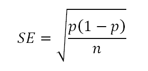
1. Standard error: This is a statistic that reflects the ‘typical’ amount of sampling error we could expect to affect our sample. As discussed above, one thing that will influence the sampling error is the size of our sample, for which we will use the symbol n. The other thing that affects the standard error is the proportion of the proportion of people who endorse the option in question, p, which can range from 0 to 1. Sampling error is greatest when p is .5 (50% support for the response) and drops off at higher and lower values. If we know these two figures and our poll aims to make inferences about a relatively large population (such as all voters in Australia), the standard error can be calculated using the following equation:

   

   Typically polls report the maximum margin of error, which is based on the standard error when p is .5. In the case of the Newspoll, putting p = .5 and n = 1123 into that equation produces a standard error of .01492, or just a shade under 1.5%.

2. Confidence level: We can decide how confident we want to be that the margin of error will be likely to capture the true population value. A common approach, and one that you can typically assume has been used when polling results fail to report the details of their margin of error, is to use a confidence level of 95%. But we could just as easily set it to another value such as, say, 90%. In that case, our margin of error would be smaller, with the trade-off that the chances that the real value could fall outside our estimated range would be higher. In the case of the Newspoll, for a 90% confidence level the margin of error would drop to around 2.5%, but then we would expect the estimated range to ‘miss’ its target in 1 out of every 10 polls rather than 1 out of 20.

   Our knowledge of the normal distribution allows us to estimate that 95% of sample statistics will be no more than 1.96 times the standard error away from (above or below) the true population value. If a different confidence level is used, there are normal distribution calculators and tables to find the corresponding value. In the case of the December Newspoll, then, the margin of error at a 95% confidence level will be 1.96 times the standard error of .01492, which is approximately equal to 2.92% – near enough to 3% that we can use it as a round figure.

   Remember that this is the maximum margin of error – with Gillard’s rating around 50%, this is a close enough estimate for the sampling error in her evaluation. But if we used the Newspoll sample’s preferred PM values for Abbott (p = .32) and uncommitteds (p = .16) when calculating the standard error, then we would estimate the margins of error on those values at around 2.7% and 2.1%, respectively.

Back to overview.

The Shortcut

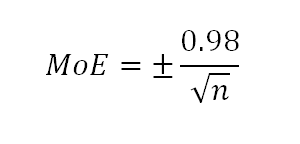
The calculations above follow the conceptual path to the margin of error. But if you ever want to calculate the margin of error as it is typically reported, there is a shortcut. At a 95% confidence level, the maximum margin of error is equal to 0.98 divided by the square root of the sample size, or:

You might notice that 0.98 is half of 1.96. This shortcut equation comes from combining the two stages of the calculations above and using a value for p of .5 – if you plug the Newspoll’s n = 1123 into the equation, you get the same margin that we found in the previous section. This shortcut gives a quick way to estimate the largest margin of error you should allow for in a poll’s results.

Back to overview.

The Implications

The risk with polling statistics is that we can overlook the uncertainty involved in sampling. People like precise figures. They’re easy to report, easy to understand and easy to compare. But the precision in those sample figures can mask their imprecision as an estimate of the population. Any time we use the sample’s responses to draw conclusions about the population – which is typically what we aim to do – we need to take into account the limits on the accuracy of our estimation. In the case of our preferred PM example, it remains clear that Gillard, whose true percentage support is likely in the low 50s, holds a lead over Abbott, whose clear support is likely somewhere in the low 30s. In this sense, our margin of error simply serves to remind us that the margin probably isn’t exactly 52 vs 32. Each of those values could be off by a few points in either direction.

If we can’t eliminate this uncertainty, how can we become more confident or precise in our estimates? Multiple estimates, such as different polls conducted in similar ways and at similar times, help with this. We can begin to look at where the ranges estimated in each poll overlap and converge on a more precise idea of where the true value is most likely to be. With federal polling relatively thin on the ground at our current point in the electoral cycle, this isn’t always feasible. Essential Research released poll results at the same time as the December Newspoll, but they didn’t measure preferred PM judgments (and fair enough, some might say). But when we do have multiple sources of data we should make use of them to refine our estimates – but we must also be careful to note differences in the methods and measures used across polls.

The potential impact of sampling error on a series of polls must also be kept in mind. When comparing any two (or even a few) data points from a poll’s results over time, it’s difficult to discriminate the possible effects of sampling error from actual changes. For instance, Gillard’s rating of 52% was down from 54% in the previous (November) poll. Does this reflect an actual drop in support or just the effect of measuring two different samples? There is a large degree of overlap in the intervals we would estimate for those two poll results. But all too often the exercise of interpreting what the latest poll shows will end up with a commentator fitting the data to their own preconceived narrative about current events. Solid analysis of shifts in public opinion really requires a decent number of data points and a focus on general trends, while continuing to factor in the unpredictability of sampling error.

Let’s finish with a few quick caveats:

• This tutorial relates only to the random variation in statistics as a result of sampling error. In other words, this focus on margin of error is an issue to do with the analysis of polls; but the meaningfulness of results will be affected by other factors as well, including issues in the design (e.g., sampling procedures) and the approach to measurement (e.g., the wording of questions and response options).
• When looking at the estimated intervals, it’s worth remembering that by definition the margin of error for one poll out of 20 will fail to capture the true value in the population. ‘Rogue polls’ are a fact of life, and outliers based on sampling error aren’t any more or less likely to happen to one pollster, or in one particular direction.
• We tend to focus on the margin of error as implying that apparent differences may really not exist, but it is equally plausible that sampling error might mask a difference that really does exist.
• The margin of error relates to individual results in the poll. You can use those margins as a rough gauge of whether differences or changes in the figures might be explained by sampling error. But formally comparing two values and making a judgment about whether the difference between them is likely to be ‘real’ and not just an effect of sampling error involves different computations to test for a statistically significant difference. That is beyond the scope of this tutorial, but see below for a useful tool that lets you compare figures within and across polls.

Back to overview.

Additional Resources

Possum has a nice gadget for calculating margins of error, interval estimates, and comparisons of two results for statistically significant change. Go and play with it, and make use of it any time new polling data comes out and you want to get a feel for what it might mean.

The bottom graph on this page by David Lane allows you to play with the normal distribution and see how many standard errors would correspond to different confidence levels.

Back to overview.

A Note

This is the first in a planned series of posts about polling methods and analysis. The idea is to give as clear and concise an explanation of the concepts, as well as some details about the computations involved – but to present the information so that people who aren’t comfortable with the statistics can skip over the maths while still learning how to think about the concepts. I will be grateful for any feedback about the usefulness of the tutorial, as well as questions about anything that is unclear or not covered.